quick report
general
seniority_list is able to rapidly generate statistical summary reports for all integrated list outcomes. This capability is provided through the functions within the reports module. Existing datasets are automatically recognized and loaded internally by the reports module through use of the load_datasets function from the functions module.
This program feature offers insight into significant outcome metrics prior to more detailed analysis using the built-in plotting functions or other techniques. The user may also find this functionality helpful for testing or validation following list modification with the editor tool.
Quick reporting trades the extensive customization and analytical resolution offered with the built-in plotting functions for a fast outline reporting of a limited set of predetermined attribute measurements.
Report output is stored within the reports/<case name> folder. The report information is presented as two excel spreadsheets and numerous chart images. Summary reports may be shared with others by simply copying and disributing the reports/<case name> folder.
A more recent addition to the reporting capability of senior_list is time-in-job comparisons, discussed in the section below. The file output from the job_diff_to_excel function is stored within the reports/<case name>/by_employee folder.
computed statistics
The reports module functions generate a collection of summary data consisting of average attribute values for each employee group over the life of the data model.
The statistics are computed in two ways:
values for employees at retirement only
annual values for all employees
The values are calculated from groupings, or bins, of certain categorical data:
longevity or date of hire year
starting job level
population quantile membership (within each employee group), with two subsets:
initial list quantile
monthly running quantile
Within the categorical groupings, the routines measure a default set of attributes:
seniority list percentage (“spcnt”)
seniority number (“snum”)
job value rank (“cat_order”)
percentage within job level (“jobp”)
career earnings (“cpay”)
grouping method definitions
longevity year or date of hire year
Employees may be grouped and compared by the longevity year or date of hire year (selectable as a function input). Grouping in this fashion permits future year comparison of employees from each employee group from the same hire year or with the equivalent longevity year.
quantile
The default number of quantiles used for membership grouping is 10, meaning an employee at 5% on the list would be a member of quantile 1, 25% would be quantile 3, etc. The number of quantiles may be modified through a function input.
initial list quantile
Employees are assigned to a quantile group based on separate employee group seniority list percentage postition at the merger date. Initial list quantile members are tracked throughout the data model time period, for each employee group separately. This tracking provides a comparative attribute value analysis for cohort list percent employees from each group. Using the initial quantile membership will allow comparing employees from separate groups in future years who were initially members of the same relative quantile.
monthly running quantile
For each month of the data model, employees are assigned to a quantile group based on separate employee group seniority list percentage postition. Running quantile members are tracked throughout the data model time period, for each employee group separately. This tracking provides a comparative attribute value analysis, averaged on an annual basis, for cohort list percent employees within each group. This style of analysis will show, for example, the average job level held by the 3rd quantile of employees within each group for the year 2022.
starting job level
Employees are assigned to a initial job level group based on separate employee group job level postitions at the merger date. Initial list job level members are tracked throughout the data model time period, for each employee group separately. This tracking provides a comparative attribute value analysis for cohort initial job level employees from each group. Using the initial job level membership will allow comparing employees from separate groups in future years who were initially members of the same relative job group.
excel files
The stats_to_excel function stores the statistical data in two excel workbooks:
ret_stats.xlsx
annual_stats.xlsx
Each workbook contains many worksheets. Each worksheet contains results for a specific calculated dataset with a certain type of grouping applied.
ret_stats.xlsx workbook
The image below is the same worksheet as the example above, with the addition of some formatting for descriptive clarity. The yellow header row contains the measured attributes, and the blue row just below contains employee group codes. The peach-colored column contains longevity year information, while the green column holds retirement year data.
This worksheet reveals average retirement attribute values for equivalent longevity year employees from each employee group. The red-boxed area shows average attribute values for employees with a 1986 longevity year retiring in year 2021. In this example, using the columns under the “spcnt” header, employees from group 2 with a longevity year of 1986 retiring in 2021 will finish at an average of 39.3% on the integrated list. This compares to 3.6% and 14% for groups 1 and 3 respectively.
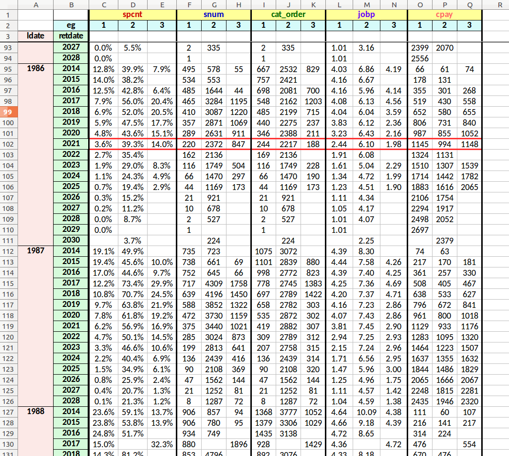
stats at retirement for each employee group tracked by longevity year membership
annual_stats.xlsx workbook
The example below has also been formatted as described above.
This worksheet reveals average annual attribute values for employees with the same intial job level at the start of the data model.
In other words, a snapshot of jobs held by all employees is taken at the very beginning of the data model. Employees within each beginning snapshot job level are then tracked throughout the entire data model time period, with average attribute measurements sampled on an annual basis. The measurements are taken for each employee group separately.
In the image below, the red-boxed area contains average attribute values for employees with an initial job level of 6, as measured in year 2022 of the data model. The boxed data under the “spcnt” header indicated that employees from group 2 will be positioned at an average of 56% on the integrated list. This compares to 26.1% and 33% for groups 1 and 3 respectively.
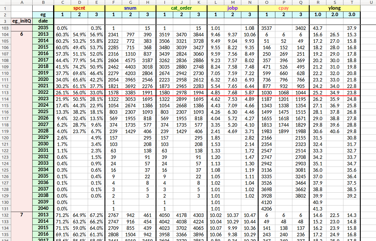
annual stats tracked by separate employee group initial quantile membership (the red-boxed area shows average attribute values in 2022 for employees who initially belonged to quantile 6)
chart images
The retirement_charts and annual_charts functions within the reports module create many simple statistical charts which are stored as image files within auto-generated folders located within the reports/<case name> folder. The chart images are visual representations of the computed statistical data.
With the default function inputs, several directories will be created within the case-specific reports folder:
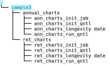
folders created with the chart creation functions
The total number of chart images stored within the annual_charts and ret_charts folders may be relatively large. With the “sample3” example case study, a total of over 2,000 chart images are produced!
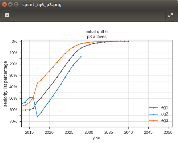
the reports module functions produce numerous charts similar to the chart above
Despite the large quantity, it is does not take long to review the charts using a standard image viewer and left and right arrow keyboard buttons. The routines that produce the charts use the same chart background, scales, and labels for all charts within a category - only the data lines and the titles change from chart to chart. This setup makes is very easy to see how measurements change between charts.
time-in-job and career pay differential report
The job_diff_to_excel report function will generate spreadsheet reports indicating differences in the number of months employees will spend working within the various job levels, and the corresponding difference in career compensation. The user may select any two outcome datasets for comparison.
By default, the generated spreadsheets will be formatted to display employee group color-coded rows and color-coded font to indicate gains or losses in the various job level categories. This formatting is very useful for visual interpretation, but does add time to the process (for reference, the “sample3” example case requires approximately 40 seconds with an i7 linux desktop computer). The formatting may be turned off to create the files more quickly.
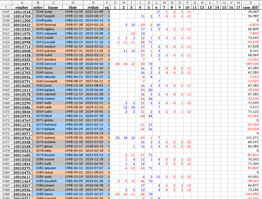
example job_diff_to_excel module function output - column width formatting must be done manually following the creation of the spreadsheet
REPORTS notebook
seniority_list includes an example notebook demonstrating the usage of the reports module functions. The datasets must be created first before attempting to generate reports.